Lorenz and modular flows: a visual introduction
A tangled tale linking lattices, knots, templates, and strange attractors.|
Etienne Ghys |
|
1.Introduction
Sometimes, seemingly unrelated objects turn out to be
related... We would like to present here a mathematical example, exhibiting a
close connection between two dynamical systems, one coming from number theory and
the other from meteorology.
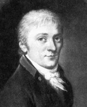 |
In 1801, Carl Friedrich Gauss published Disquisitiones Arithmeticae, his first masterpiece. It deals with the foundations of the theory of number fields. Today, many important aspects of this theory can be expressed in terms of a dynamical system acting in the space of lattices: the modular flow.
|
 |
We would like to describe a close topological connection between these two mathematical objects.
This article cannot be qualified as mathematical
since it contains no proof! Our main motivation is in the visualization of some
of the marvelous mathematical objects which are involved. We have tried to explain
enough mathematics, at a rather elementary level, to comment on the pictures and
clips which are the true content of this e-paper.
Our story is organized in a very simple way. First we
describe the Lorenz attractor (2.1) and its template (2.2), then
the space of lattices (3.1), the modular dynamics (3.2) and
its periodic orbits (3.3), and finally we establish
a connection (4.1 and 4.2) between these two dynamical systems!
This is the result of the collaboration of a mathematician and an artist-geometer. The reader may consult
[1] for more mathematics, and [2] for more graphics.
Graphics were made in Ultrafractal
[13] and Povray [14]. Data for knot
drawings were extracted from Knotplot [12]. Larger versions of the films can be seen at
Jos Leys' site.
 button, or, as the case may be, by clicking on
a specific picture. (Linux based browsers may be an exception, for which we apologize).
button, or, as the case may be, by clicking on
a specific picture. (Linux based browsers may be an exception, for which we apologize).Copyright for all films and images is by Jos Leys / Etienne Ghys.
2.The Lorenz flow
2.1 The Lorenz strange attractor and its periodic orbits
The model discovered by E. Lorenz is described by the following differential equation in 3-space [3]:
|
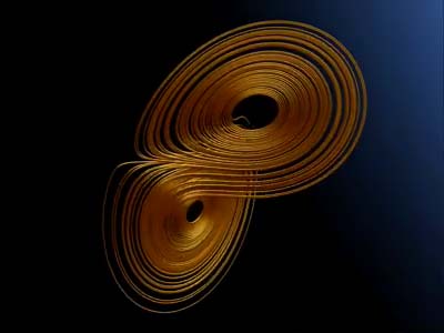
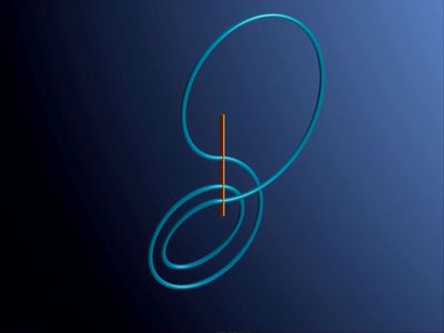
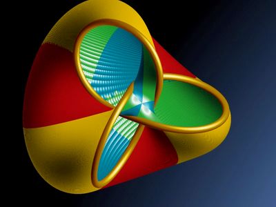
When Lorenz plotted the trajectories of this differential equation on his primitive computer, he could see something like the picture on the right (click on the image for a movie) : The amazing fact is that this picture is robust. If we perturb the equation, the phenomenon persists: trajectories tend to approach a set which is now called a strange attractor. We shall not try to discuss here the relevance of this object to fluid dynamics, but it happens that the Lorenz attractor has become one of the most paradigmatic symbols in modern dynamical systems, an icon of chaos theory (see for instance [4]). |
|
|
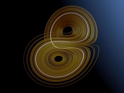
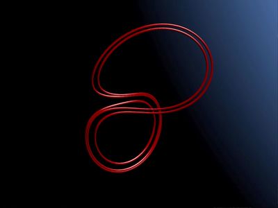
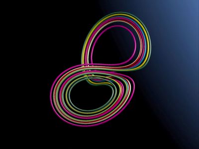
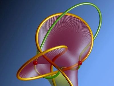
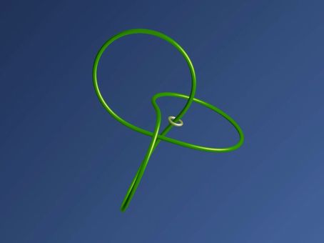
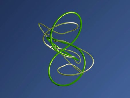
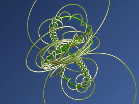
In the 1980s, Joan Birman and Bob Williams made the simple but crucial observation that a periodic orbit of a vector field in 3-space is a closed embedded curve which therefore defines a knot. They suggested that the study of the topology of the knots appearing in the Lorenz equation could yield some understanding of this important dynamical system [5]. The pictures below show some of the periodic orbits that one finds in the Lorenz equation. | ||||||||
 |
 |

| ||||||
|
Some of these knots look topologically trivial, but some are non trivial, like the red orbit which turns out to be a trefoil knot. One of the motivations of Birman and Williams was that these periodic orbits seem indeed to give a good approximation of the attractor. In the picture on the right (click on it for a movie), one sees simultaneously a collection of closed orbits, suggesting that the attractor is some kind of limit of its periodic orbits. In a way, one could think of the attractor as an infinite link with infinitely many components. |
|
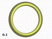
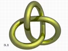
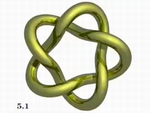
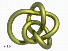
Birman and Williams proved that Lorenz knots are indeed very interesting, at the same time rich enough and very peculiar. Rather than stating technical results concerning Lorenz knots, let us limit ourselves to some numerical statements. Recall that a knot is simply a closed curve in space with no double point, and that one says that two knots are the same, or are equivalent, if one can go from the first to the second through a continuous deformation without creating intersection points (see for instance [6], [7], [8]). One crude way of classifying knots is to order them according to their crossing number, which is the minimum number of intersections of a projection of a representative of the given knot. One knows for instance that there are 250 (prime) knots with 10 crossings or fewer. It follows from the work of Birman and Williams that among those 250, only the following 8 knots appear as periodic orbits of the Lorenz attractor.
Click on the knot images below for a movie. (Knots are usually associated to a code like 8.19, meaning the 19th knot among those which can be represented in a diagram with 8 crossings, using an ordering which is more traditional than logical).
|
|
|

|
|

|
|

|
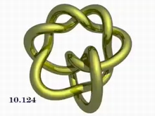
Among the 1 701 936 (prime) knots with 16 crossings or less , only 21 appear as Lorenz knots (checked using a computer and [17]).
|
Some are rather interesting like the knot 'Non-Alternating 12.725' with 12 crossings: |
|
|
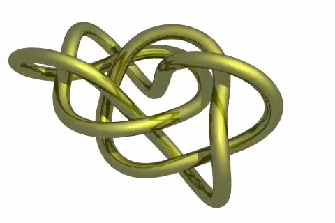
As a sample counter-example, the figure eight knot is not a Lorenz knot. |

|
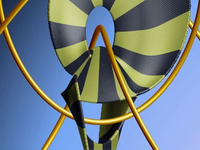
2.2 The Lorenz template
|
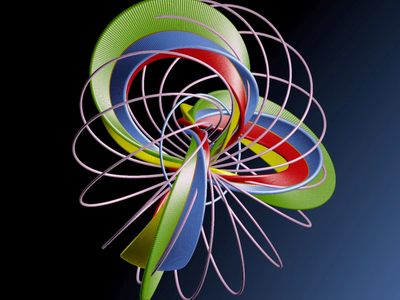
How can one prove such facts? One deals with a combinatorical model of the Lorenz equation which is easier to analyze. First, one constructs the so-called Lorenz template in a way described by the following pictures. | ||||||||
 |
 |
| ||||||
|
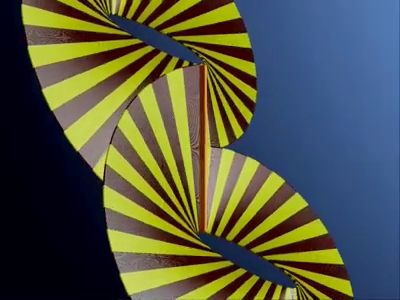
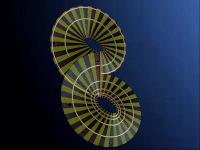
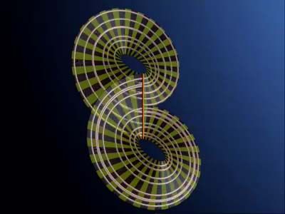
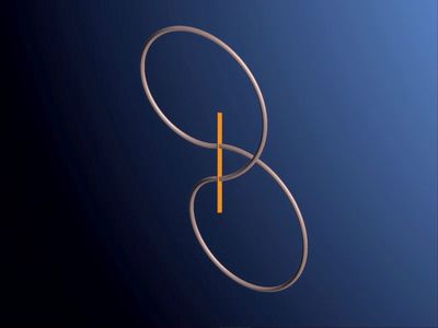
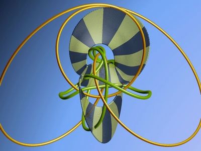
Consider two bands of paper, and unfold them in space as shown in the clip. This produces a two dimensional object in space which is a branched surface: this is the Lorenz template. The branching locus is the vertical segment that one sees in the middle of the picture. On this template, there is a rather natural dynamical system, which is shown on the following pictures. | ||||||||
 |
 |
| ||||||
|
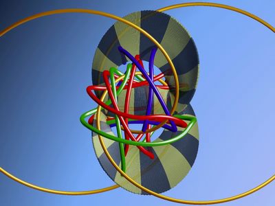
If we identify the vertical segment with the interval [0,1], then each orbit traverses the template in such a way that the point with coordinate x comes back to the interval at the point 2x mod Z. Therefore if one looks for periodic orbits, we have to look for periodic points of the doubling map from the interval to itself. For instance, the doubling map sends the point 1/3 to 2/3, and then back to 1/3 = 4/3 - 1. So, the point 1/3 is periodic of period 2, and yields a closed orbit on the template, going once in one ear of the template, and once in the other one. The following pictures show several of these periodic orbits on the template. | ||||||||
 |
 |
| ||||||
As a matter of fact, it is not difficult to describe these periodic orbits by an itinerary, which consists in a finite sequence of symbols, say left and right. For any such sequence, there is exactly one periodic orbit which follows this itinerary, going successively in the left and right wings of the template, in the order given by the itinerary. Conversely, the periodic orbit defines the itinerary, up to a cyclic permutation which amounts to choosing a starting point. In this way, one can imagine a study of the topology of the Lorenz knot associated to a given itinerary. This is what Birman and Williams did. The fact that this geometric Lorenz attractor does describe the original Lorenz equation has been established much more recently by Tucker [9],[10].
3. The modular flow
3.1 The space of lattices and its topology
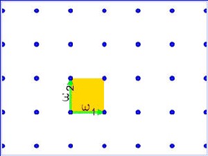
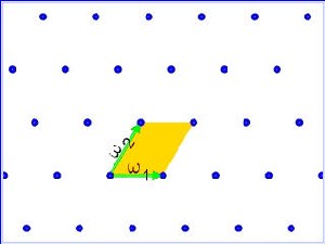
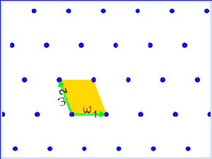
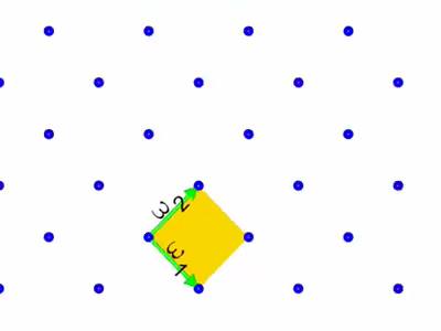
Given two linearly independent vectors ω1 , ω2 in the plane, one can consider the subgroup L of R2 that they generate:
L= {n1ω1 + n2ω2| n1
, n2
![]() Z}.
Z}.
|
|
|
A subset of the plane of this form is called a lattice. Of course, the same lattice L can be generated in many ways by two vectors. If a, b, c, d are integers such that ad−bc= ±1, the vectors aω1+ bω2 and cω1+ dω2 generate the same lattice.
The set of lattices is a topological space: one says that two lattices are close if they can be generated by pairs of vectors in the plane which are close. This space has been studied for many years by mathematicians, starting with the great Gauss in his Disquisitiones Arithmeticae (1801), in which he discussed in depth the arithmetical theory of integral quadratic forms.
Think of the plane R2as the complex plane C. For each lattice L, one can define two complex numbers
 ;
;  .
.
It is easy to check that these series converge since the exponents 4 and 6 are bigger than 2. Now, an odd exponent would yield a zero sum, since the lattice is obviously symmetric with respect to the origin, so that 4 and 6 are indeed the first cases to consider. As for the 60 and 140, they are normalizing constants which are not relevant to our discussion. The main point is that the pair of complex numbers ( g2(L) , g3(L) ) characterizes the lattice. More precisely, a pair of complex numbers (g2, g3) corresponds to a lattice if and only if the so-called discriminant Δ = g23− 27g32 is not zero. See for instance [11], [16] for a proof.
Summing up, the space of lattices can be identified with the complement in C2 of the curve Δ = 0.
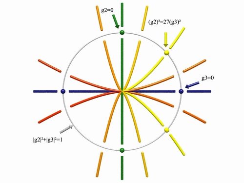 The picture on the left represents symbolically C2.
Keep in mind that C2 is R4, so that this is a four dimensional picture! The horizontal
blue axis corresponds to those lattices for which g3=0; this is a
copy of C=R2. The vertical green axis corresponds to those
lattices for which g2=0; this is another copy of C=R2. The
yellow curve represents Δ=0, but again this
is a one dimensional curve over the complex numbers, and therefore a surface
from the point of view of real numbers.
The picture on the left represents symbolically C2.
Keep in mind that C2 is R4, so that this is a four dimensional picture! The horizontal
blue axis corresponds to those lattices for which g3=0; this is a
copy of C=R2. The vertical green axis corresponds to those
lattices for which g2=0; this is another copy of C=R2. The
yellow curve represents Δ=0, but again this
is a one dimensional curve over the complex numbers, and therefore a surface
from the point of view of real numbers.
How can we look at this four dimensional object in a concrete way? If L is a lattice and k a non zero real number, one can look at the lattice kL, which is just the same as L, but rescaled by a factor k. This suggests restricting our attention to those lattices whose fundamental domain has area 1, or still in other words, those generated by two vectors ω1, ω2 defining a parallelogram of area 1. Note that
g2(kL) = k−4g2 (L) ; g3(kL) = k− 6g3(L),
so that for each lattice L one can find a unique k > 0 such that |g2(kL)|2+ |g3(kL)|2= 1.
|
This means that if we want to restrict our study to
lattices up to rescaling, or to lattices of area 1, we have to look at the
complement in the unit sphere |g2|2+ |g3|2= 1 of
the zero set of Δ. This unit sphere
is 3-dimensional, and the zero set intersects it in a one dimensional object,
which turns out to be a trefoil knot. The 3-sphere is easier to visualize than C2. If one chooses
a point in a sphere, one can project from that point to the tangent space at the
opposite point: this is the so-called stereographic
projection, illustrated in the following picture for the two dimensional case
(the Riemann sphere). |
 |
Hence the space of lattices of area 1 is identified with the complement of a trefoil knot in the 3-sphere, which, after deleting one point, is the complement of a trefoil knot in the usual 3-space. So, there is some hope of seeing something! Lets have a look.
|
This picture (click it for a movie) shows the 3-sphere, or better, its stereographic projection in 3-space, or, even better, the projection to your 2-dimensional screen of this stereographic projection. As the film evolves, the point from which the projection is done is moving continuously so that you can admire the whole scene! In blue (resp. green), the coordinate axis g2=0 (resp. g3 =0) which intersects the sphere in a circle, which is seen from time to time as a straight line when the source of the projection is on this circle. As for the yellow trefoil knot, it is the intersection of the zero set of Δ with the sphere. |
To get more topological insight, lets have a look at some additional structures in the space of lattices of area 1.
|
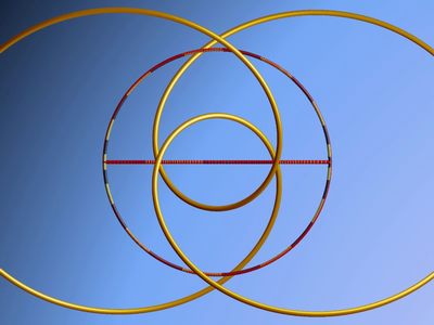
Given a lattice L and angle θ ∈ [0,π[, one can rotate the lattice by θ in the plane. One gets another lattice Lθ. As θ goes from 0 to π, this describes a circle in the space of lattices. Note that if θ ≠ 0, the two lattices L and Lθ are different in general, with only two exceptions. If L is a square lattice, it is equal to its image by rotations by π/2 and if L is a regular hexagonal lattice, it is equal to its image by rotations by π/3 and 2π/3. All this implies that the space of lattices of area 1 is filled by circles corresponding to the orbits of these rotations. These circles are only topological circles; in fact they are themselves trefoil knots with the exceptions of the two special cases that we mentioned which are shorter (they close after π/2 and π/3 instead of π) and which turn out to be round circles. As a matter of fact, these circles are just the blue and green circles that we previously met. This decomposition of the 3-sphere into a collection of trefoil knots and two circles is an example of a Seifert fibration. See the picture on the right (click on it for a movie): |
|

|
There is an additional structure in the 3-sphere, so to speak dual to the Seifert fibration. We know that to each lattice is associated a non zero complex number Δ. If one multiplies a lattice by a real number k > 0, this Δ is multiplied by k−12 so that the argument is preserved. This suggests looking at the decomposition of the space of lattices of area 1 according to the value of the argument of the complex number Δ. The set of lattices of area 1 for which Δ has a given argument defines a surface in the 3-sphere whose boundary is the trefoil. The picture on the left (click it for a movie) shows of one of these Seifert surfaces. |
|
Of course, we get one of these surfaces for each value of the argument of Δ. If this argument describes a full turn, the corresponding Seifert surfaces will sweep around all 3-space, always keeping the same boundary. For some value of the argument, the Seifert surface passes through the pole of the stereographic projection, so that the surface seems to be infinite at that instant. (Click on the picture) |
|

|
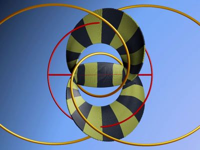
To understand this fibration
of the complement of the trefoil knot,
lets delete a part of the Seifert surfaces, and lets look at the motion in
the neighbourhood of the trefoil knot. The following clip shows parts of four
Seifert surfaces, corresponding to four values of the argument, rotating around
the trefoil. Topologists say that the 3-sphere is an open book, that
the trefoil is the binding, and that the Seifert surfaces are the pages.
|
Now, for the fun of it, lets have a look at the global picture, including the trefoil, the axis, the Seifert fibers, and the Seifert surfaces, all together! (Click on the picture for a movie)
 |
3.2 The Modular dynamics
Now that we have a clear topological idea of the space of lattices of area 1, we can define a dynamical system on that space. The definition is very simple. For every real number t, consider the matrix
 .
.
If L is a lattice of area 1, its image ![]() by the matrix
by the matrix ![]() is again a lattice of area 1.
This defines a dynamical system in the space of lattices of area 1 which is called the modular flow. The trajectory
of the lattice L is the curve described in the space of lattices by
is again a lattice of area 1.
This defines a dynamical system in the space of lattices of area 1 which is called the modular flow. The trajectory
of the lattice L is the curve described in the space of lattices by ![]() as the time t describes the real numbers.
as the time t describes the real numbers.
Our purpose is to give a visual description of this flow and of its periodic orbits. This flow is a well known example of an Anosov flow which means that there are stable and unstable directions. Let us explain this. Introduce two other flows by
 ;
;
 .
.
Note that ![]() and
and ![]() ,so that if one takes two lattices L and
,so that if one takes two lattices L and
![]() (resp. L and
(resp. L and
![]() ) and if one looks at their future (resp. their past)
in the modular flow, i.e. if one looks at their images by
) and if one looks at their future (resp. their past)
in the modular flow, i.e. if one looks at their images by ![]() with t positive (resp. negative), then the two lattices tend to approach exponentially fast. One says
that L and
with t positive (resp. negative), then the two lattices tend to approach exponentially fast. One says
that L and ![]() (resp.
(resp.
![]() ) are in the same stable (resp. unstable) curve.
) are in the same stable (resp. unstable) curve.
|
The pictures below explain this situation. At first, one sees an initial point L, and two arcs in the stable
and unstable manifolds, i.e. two intervals | ||||||||
 |
 |
| ||||||
3.3 Periodic orbits and their linking with the trefoil
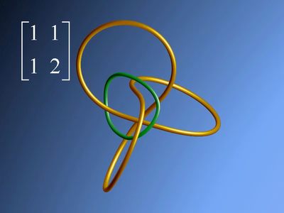
We can now start the topological description of the periodic orbits of the modular flow. There is a simple way to describe these periodic orbits. Consider a 2 × 2 matrix A with integral coefficients and determinant 1:
 .
.
Clearly, the matrix A preserves the standard square lattice Z2 in R2. Suppose that A is hyperbolic, which means that |a + d| > 2 in which case A is diagonalizable over the real numbers. In this case, one can find a 2×2 matrix P such that

for some t (note that the product of the two eigenvalues of A is 1). So, if we define the lattice L
to be the image of Z2 by P, one finds that L is fixed by
![]() .
In this way, for each integral matrix with determinant 1, we find a fixed point for
.
In this way, for each integral matrix with determinant 1, we find a fixed point for
![]() for some t
, i.e. a periodic orbit of the modular flow. Note that the period of this periodic orbit is t
, which is the logarithm of the absolute value of an eigenvalue of A.
for some t
, i.e. a periodic orbit of the modular flow. Note that the period of this periodic orbit is t
, which is the logarithm of the absolute value of an eigenvalue of A.
Hence every hyperbolic matrix A defines a periodic orbit of the modular flow.
The following periodic clip (click it to run) shows a periodic orbit in the space of lattices of area 1. Note that each point follows
a hyperbola, the orbit of ![]() in the plane, so
that the trajectories of the points are not periodic, but the trajectory of the lattice, as a part of the plane, is indeed
periodic.
in the plane, so
that the trajectories of the points are not periodic, but the trajectory of the lattice, as a part of the plane, is indeed
periodic.
 |
It is not difficult to see that if one replaces A by ± BAB−1 where B is some other integral matrix with determinant 1, one gets the same periodic orbit.
There is a natural bijection between periodic orbits of the modular flow and conjugacy classes of hyperbolic integral matrices of determinant 1, up to sign.
These periodic orbits have a very old mathematical tradition. One finds them in many different areas, in different disguises: closed geodesics on the modular surface, equivalence classes of integral indefinite quadratic forms, ideal classes in quadratic number fields, continued fractions etc.
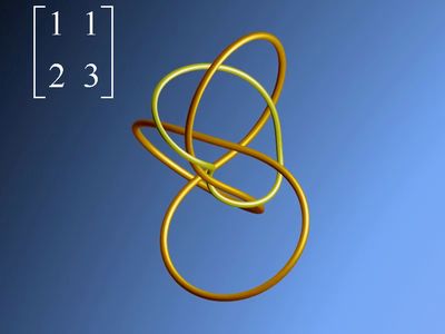
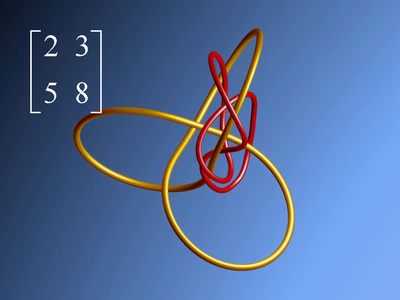
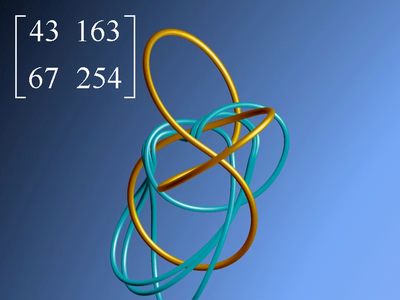
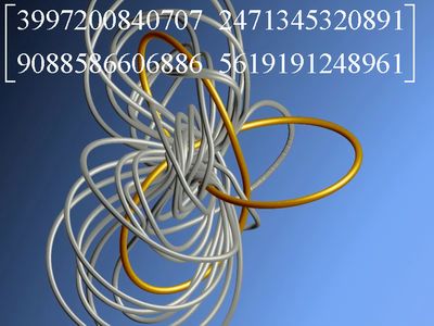
Each one of these periodic orbits is a closed curve in the space of lattices of area 1, hence defines a knot in the complement of the trefoil knot. We wish to investigate these modular knots from the topological point of view. Let us first look at some examples.
 |
 |
 |
 |
 |
 |
|
|
For the matrix  the knot looks
disappointing! It is a small trivial knot. . . For the matrix
the knot looks
disappointing! It is a small trivial knot. . . For the matrix
 the knot is
still trivial but placed differently with respect to the trefoil. For the matrix
the knot is
still trivial but placed differently with respect to the trefoil. For the matrix
 the knot is more
interesting; it is a trefoil knot. For the matrix
the knot is more
interesting; it is a trefoil knot. For the matrix  it is a torus knot T(4, 5). For the matrices
  and
and
 it is, well, more complicated!
Before we discuss the nature of these knots, let us ask a seemingly simpler question:
Given a hyperbolic integral matrix A with determinant 1, denote by kA the associated knot. Can one compute the linking number between kA and the trefoil knot?
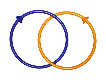
One should quickly recall the notion of linking number of two disjoint oriented knots in 3-space (also introduced by Gauss in the very different context of electromagnetism). Suppose that two oriented knots k1 (blue) and k2 (orange) do not intersect, and project them onto a plane in a generic way. These projections need not be disjoint of course.
|
|
|
|
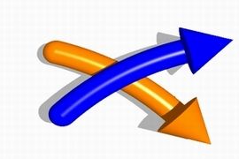
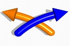
Let us consider the points where the projection of k1, the blue knot, crosses once over the projection of k2, the orange knot. These crossing points may have two local behaviors, as shown in the pictures on the left. |
Attach the sign +1 to the left situation and −1 to the right one, and sum these indices over the set of all crossings of k1 over k2. The result is called the linking number between k1 and k2. For instance, in the knot picture on the left, the blue curve crosses once over the orange one, with a '+1' sign, so that the linking number is '+1'. In the picture on the right, one has two cross-overs with different signs, so that the linking number is 0.
The important point is that this number is independent of the (generic) projection used to compute it, and remains invariant if the knots move continuously without intersecting each other.
Now, let us come back to our question, and try to compute the linking number between kA
and the trefoil knot. Recall that the trefoil knot is the boundary of a Seifert surface where the argument of Δ is equal
to some fixed value, for instance 0 (which corresponds to Δ being a positive real number). Given a closed oriented curve
![]() in the
complement of the trefoil knot, one can consider its image by the Δ map,
and one gets a closed curve in the complex plane which avoids the origin.
Clearly, the linking number between
in the
complement of the trefoil knot, one can consider its image by the Δ map,
and one gets a closed curve in the complex plane which avoids the origin.
Clearly, the linking number between ![]() and the trefoil
is the index of this closed curve with respect to the origin, i.e. the number of turns it makes around the
origin. A way to compute this index is to compute the algebraic intersection with the real axis, counting a '+1' or a '
−1' for each intersection according to whether the curve crosses from negative to positive imaginary part, or the other way.
Topologically, this means that the Seifert surface is two-sided, and that one wishes to compute the algebraic intersection of
kA with the Seifert surface.
and the trefoil
is the index of this closed curve with respect to the origin, i.e. the number of turns it makes around the
origin. A way to compute this index is to compute the algebraic intersection with the real axis, counting a '+1' or a '
−1' for each intersection according to whether the curve crosses from negative to positive imaginary part, or the other way.
Topologically, this means that the Seifert surface is two-sided, and that one wishes to compute the algebraic intersection of
kA with the Seifert surface.
This is described by the pictures below. For a given matrix A, one draws at the same time a Seifert surface and the knot kA. As the construction of kA evolves, it intersects the surface from time to time, positively or negatively. The linking number we are looking for is the sum of these signs. In the first instance, we get two plus signs, in the second instance, one plus sign, and two plus signs and one minus sign in the final one .
 |
 |
| |||||||
It turns out that there is a nice formula for computing this linking number which relates it to a famous arithmetical function.
Consider the two matrices
U=![]() ; V=
; V= ![]() .
.
As it turns out, any integral matrix A with determinant 1 is conjugate, up to sign, to a product of Us and Vs. For instance:
A=  = UVVVUUVVVUUUUV
The word in U and V is uniquely defined up to a cyclic permutation. For each matrix A, one can therefore define R(A) as the number of factors equal to U, minus the number of factors equal to V. This invariant of the matrix A will be called the Rademacher invariant of A. One of the results in [1] is the following:
Theorem: The linking number between kA and the trefoil knot is equal to the Rademacher invariant of A.
We can only refer to [1] for several proofs and more information, but in the next section we shall provide some interpretation.
4 Lorenz and modular knots
4.1 The modular template
So far we have discussed the periodic orbits in the Lorenz attractor, the Lorenz knots, and the periodic orbits of the modular flow, the modular knots.
Theorem: Lorenz knots and modular knots coincide.
More precisely, for every modular knot kA, one can deform it in 3-space to make it coincide with one of the periodic orbits of the Lorenz attractor, and conversely. Unfortunately, we cannot provide a proof here, and we will only show these deformations using some images and movies!
|
The first step of the proof consists in the construction of a modular template inside the space of lattices of area 1, which looks like the Lorenz template. We begin by constructing a one dimensional object consisting of two parts. The space of hexagonal lattices of area 1 is a circle, that we have already met as one of the axes in our description of the space of lattices: this is our first part.The second part consists of all lattices with a fundamental domain having the shape of a horizontal rhombus with inner angles between π/3 and 2π/3 Stated differently, one looks at lattices generated by two vectors which are symmetric with respect to the x-axis and which make an angle between π/3 and 2π/3 (and which are of determinant 1). This defines an interval since the angle can vary in [π/3, 2π/3]. Note that when this angle is equal to π/3 or 2π/3, the corresponding lattice is hexagonal so that this interval connects two points of the circle of hexagonal lattices. As a matter of fact, this interval is nothing more than a diameter. (Click the image on the right for a movie) |
|
|
The picture on the right shows this part of the construction. It starts with two rotations (one in 4-space and one in 3-space ) to place the trefoil knot in a convenient position, and then shows the construction of the circle and its diameter, that we have just described. (Click on the image) |
|
We then extend this one dimensional object in the unstable direction to create a two dimensional template. One would need more technical details to give a full description, but we will limit ourselves to images showing the progressive development of the template. Note however that we are discussing topology, so that this construction is far from being unique, and we have made some specific choices for visual reasons.
 |
 |
| |||||||
Now the next task is to deform one of the modular knots in the complement of the trefoil knot, so that after the deformation, the knot lies on the template exactly like Lorenz knots. Again, we cannot give details and we refer to [1] for more. The general idea is to compress the space of lattices of area 1 to a small neighborhood of the one dimensional object, by using an old idea (again of Gauss !): given a lattice L, one seeks the shortest non zero vector v in L, which is usually unique up to sign, unless the lattice has a fundamental domain with the shape of a rhombus. Then one looks for the shortest vector w in L which is not proportional to v. These two vectors v ,w define a preferred basis of L. Now, one shortens w progressively while increasing the length of v , keeping the determinant constant equal to 1. Rather than going into details, let us look at some images showing the deformation of several modular knots until they are in a Lorenz position.
 |
 |
 |
 |
 |
 |
|
|
4.2 Two final remarks
A final comment. We know that a Lorenz periodic orbit is coded by a finite list of symbols left and right expressing the itinerary of the orbit, visiting successively the left and right ears of the Lorenz template. One can check that if one associates to an orbit the product A of the matrices U and V in the same order as the left and right, then the above deformation identifies the Lorenz knot with the modular knot kA. Now, one sees that the right ear has linking number +1 with the trefoil and the left ear has linking number −1.
It follows that the linking number of kA with the trefoil is equal to the number of U letters minus the number of the V letters in the word expressing A. This is one approach to the proof of the first theorem that we mentioned: the linking number of A and the trefoil is Rademachers number.
A final treat. The modular flow is not the only remarkable
dynamical system on the space of lattices of area 1. One can also look at the
dynamics generated by the matrices ![]() that we have already
met as stable manifolds. This flow is classically called the horocyclic flow.
One would need many clips to picture the wonderful dynamics of this flow, but we shall restrict to just one, describing the periodic
orbits. Fix real numbers t and s, and consider the lattice Ls,t generated by the two complex
numbers exp(t) and s.exp(t) + i exp(−t). Fixing t and letting s run from 0 to 1,
we get a periodic curve ct in the space of lattices of area 1, which is a
periodic orbit of
that we have already
met as stable manifolds. This flow is classically called the horocyclic flow.
One would need many clips to picture the wonderful dynamics of this flow, but we shall restrict to just one, describing the periodic
orbits. Fix real numbers t and s, and consider the lattice Ls,t generated by the two complex
numbers exp(t) and s.exp(t) + i exp(−t). Fixing t and letting s run from 0 to 1,
we get a periodic curve ct in the space of lattices of area 1, which is a
periodic orbit of ![]() . The following clip shows this curve
ct when t describes some interval. When t is a large negative number, the curve c
t is a small trivial loop going once around the trefoil knot. When t is a big positive number the curve
ct gets longer and in the limit fills the whole space.
. The following clip shows this curve
ct when t describes some interval. When t is a large negative number, the curve c
t is a small trivial loop going once around the trefoil knot. When t is a big positive number the curve
ct gets longer and in the limit fills the whole space.
 |
 |
 |
 |
|
|
It is known that the the family of curves ct tends to fill the space in a uniform way but the quantitative estimate of the velocity of this phenomenon is equivalent to the famous Riemann hypothesis, one of the most enticing open questions in mathematics! [15]
References
[1] GHYS, E.: Knots and Dynamics, to appear in the proceedings of the International Congress of Mathematicians, Madrid 2006.
[2] LEYS, J.: Mathematical Imagery. http://www.josleys.com
[3] LORENZ, E.: Deterministic Nonperiodic Flow. J. Atmos. Sci.20, (1963), 130-141.
[4] VIANA, M.: Whats New on Lorenz Strange Attractors. Math. Intell. 22,(2000), 6-19.
[5] BIRMAN, J. & WILLIAMS, R.: Knotted periodic orbits in dynamical systems.I. Lorenzs equations. Topology 22(1983), no.1, 4782.
[6] ADAMS, C.: The knot book. An elementary introduction to the mathematical theory of knots. Revised reprint of the 1994 original. American Mathematical Society, Providence, RI, 2004. xiv+307 pp.
[7] KAUFFMANN, L.:On knots. Annals of Mathematics Studies 115 Princeton University Press, Princeton, NJ,(1987).
[8] SOSSINSKY, A: Knots. Mathematics with a twist. Translated from the 1999 French original by Giselle Weiss. Harvard University Press, Cambridge, MA, 2002. xxii+127 pp.
[9] STEWART, I : The Lorenz Attractor Exists. Nature 406 (2000), 948-949.
[10] TUCKER, W.: A rigorous ODE solver and Smales 14th problem. Found.Comput. Math. 2 (2002), no. 1, 53117.
[11] SERRE, J.-P.: A course in arithmetic. Translated from the French. Graduate Texts in Mathematics, No. 7. Springer-Verlag New York, Heidelberg, 1973. viii+115 pp.
[12] SCHAREIN, R.: Knotplot : http://www.pims.math.ca/knotplot/KnotPlot.html
[13] SLIJKERMAN, F. :Ultrafractal : http://www.ultrafractal.com
[14] POVRAY: Public domain raytracing software http://www.povray.org/
[15] SARNAK, P.: Asymptotic behavior of periodic orbits of the horocycle flow and Eisenstein series. Comm. Pure Appl. Math. 34 (1981), no. 6, 719739.
[16] McKEAN, H. & MOLL, V.: Elliptic curves. Function theory, geometry, arithmetic.Cambridge University Press, Cambridge, 1997.
[17] THE KNOT ATLAS.: http://katlas.math.toronto.edu/wiki/Main_Page